#climatechangecrochet – The global warming blanket.

Q. What do you get when you cross crochet and climate science?

A. A lot of attention on Twitter.

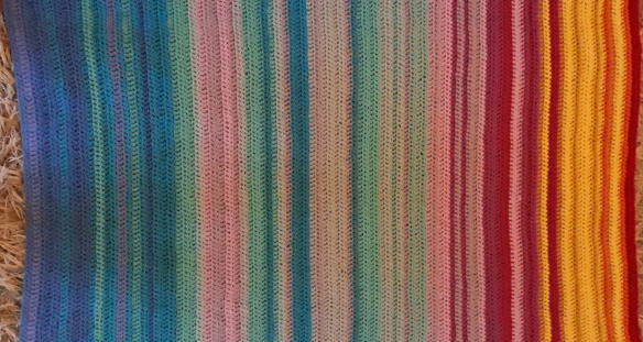
At the weekend I like to crochet. Last weekend I finished my latest project and posted the picture on Twitter. And then had to turn the notifications off because it all went a bit noisy. The picture of my “global warming blanket” rapidly became my top tweet ever, with more retweets and likes than anything else. Apparently I had found a creative way to visualise trends in global mean temperature. I particularly liked the “this is the most frightening knitwear I have seen all year” comment. Given the interest on Twitter I thought I had better answer a few of the questions in this blog. Also, it would be great if global warming blankets appeared all over the world.

How did you get the idea?

The global warming blanket was based on “temperature” blankets made by crocheters around the world. Their blankets consist of one row, or square, of crochet each day, coloured according to the temperature at their location  . They look amazing and show both the annual cycle and day-to-day variability. Other people make “sky” blankets where the colours are based on the sky colour of the day – this results in a more muted grey-blue-white colour palette. UPDATE – IN 2022 I became aware that a  global temperature blanket had been produced by Joan E Sheldon, an estaurine scientist and weaver in 2015 and a pattern made available on Ravelry in 2017. I had not seen this when I made my blanket, but I always thought there would likely be others out there in the textiles world. If you are here looking for the first “climate stripes” manifestation, it would be hers. )

I wondered what the global temperature series would look like as a blanket. Also, global warming is often explained as greenhouse gases acting like a blanket, trapping infrared radiation and keeping the Earth warm. So that seemed like an interesting link. I also had done several rainbow themed blankets in the past and had a lot of yarn left that needed using.

Where did the data come from?

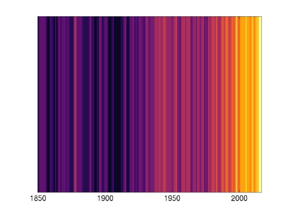
I used the annual and global mean temperature anomaly compared to 1900-2000 mean as a reference period as available from NOAA https://www.ncdc.noaa.gov/cag/time-series/global/globe/land_ocean/ytd/12/1880-2016. This is what the data looks like shown more conventionally.

globalwarmingblanketgraph

I then devised a colour scale using 15 different colours each representing a 0.1 °C data bin. So everything between 0 and 0.099 was in one colour for example. Making a code for these colours, the time series can be rewritten as in the table below. It is up to the creator to then choose the colours to match this scale, and indeed which years to include. I was making a baby sized blanket so chose the last 100 years, 1916-2016.

closeup.png

1929              1940-46        1954-56                                       1991/2  1997/8

If you look closely you can see the 1997-1998 El Nino (relatively warm yellow stripe), 1991/92 Pinatubo eruption (relatively cool pink year) as well as cool periods 1929, and 1954-56 and the relatively warm 1940-46. Remember that these are global temperature anomalies and may not match your own personal experience at a given location!

Because of these choices, and the long reference period, much of the blanket has relatively muted colour differences that tend to emphasise the last 20 years or so. There are other data sets available, and other reference periods and it would be interesting to see what they looked like. Also the colours I used were determined mainly by what I had available; if I were to do another one, I might change a few around (dark pink looks too much like red in the photograph and needed a darker blue instead of purple for the coldest colour), or even use a completely different colour palette – especially as rainbow colour scales aren’t great as they can distort data and render it meaningless if you are colour blind Ed Hawkins kindly provided me with a more user friendly colour scale which I love and may well turn into a scarf for myself (much quicker than a blanket!).

IMG_20170612_183501

How can I recreate this?

If you want to create something similar, you will need 15 different colours if you want to do the whole 1880-2016 period. You will need relatively more yarn in colours 3-7 than other colours (if, like me you are using your stash). You can use any stitch or pattern but since you want the colour changes to be the focus of the blanket, I would choose something relatively simple. I used rows of treble crochet (UK terms) and my 100 years ended up being about 90 cm by 110 cm. You can of course choose any width you like for your blanket, or make a scarf by doing a much shorter foundation row. It goes without saying that it could also be knitted. Or painted. Or woven. Or, whatever your particular craft is.

table

How long did it take?

I used a very simple stitch, so for a blanket this size, it was a couple of months (note I only crochet in the evenings 2 or 3 evenings a week for a couple of hours with more at some weekends). It helped that the Champions League was on during this time as other members of the household were happy to sit around watching football whilst I crocheted. Weave the ends in as you go. There are a lot of them, and I had to do them all at the end. The time flies because….

Why do I crochet?

I like crochet because you can do simple projects whilst thinking about other things, watching TV or listening to podcasts, or, you can do more complicated things which require your full attention and divert your brain from all other things. There is also something meditative about crochet, as has been discussed here (https://www.theguardian.com/lifeandstyle/2013/may/16/knitting-yoga-perfect-bedfellows) I find it a good way to destress. Additionally, a lot of what I make is for gifts or for charities and that is a really good feeling.

What’s next?

Suggestions have come in for other time series blankets e.g. greys for aerosol optical depth punctuated by red for volcanic eruptions, oranges and yellows punctuated by black for solar cycle (black being high sun spot years), a central England temperature record. Blankets take time, but scarves could be quicker so I might test a few of these ideas out over the next few months. Would love to hear and see more ideas, or perhaps we could organise a mass “global warming blanket” make-athon around the world and then donate them to communities in need.

And finally.

More seriously, whilst lots of the initial comments on Twitter were from climate scientists, there are also a lot from a far more diverse set of folks. I think this is a good example of how if we want to reach out, we need to explore different ways of doing so. There are only so many people who respond to graphs and charts. And if we can find something we are passionate about as a way of doing it, then all the better.

Three women meteorologists for International Women’s Day 2017

On International Women’s Day 2017 I could write about famous women that lots of people (although still not enough) already know about. I could write honouring the wonderful women in my life, but other social media platforms are the way to do that. Instead I would like to introduce you to three influential voices of women in Meteorology, recognising my multiple work roles as a climate scientist, President of the Royal Meteorological Society and Dean for Diversity and Inclusion. Forgive the length of the post, there is so much to say about each!

Eunice Foote (1819-1888) was both a scientist and a proponent of women’s rights. As has come to light over only the past few years (work by Sorenson in 2011, and more recently Katherine Hayhoe), Foote conducted early work on what we now call the greenhouse effect. The experiments investigated the warming effect of the sun on air, including how this was increased by carbonic acid gas (carbon dioxide), and bear a striking resemblance to some outreach experiments still used today. She also speculated on how an atmosphere of this gas might affect climate. “An atmosphere of that gas would give to our earth a high temperature; and if as some suppose, at one period of its history the air had mixed with it a larger proportion than at present, an increased temperature from its own action as well as from increased weight must have necessarily resulted.”

Her paper “Circumstances affecting the heat of the sun’s rays,” was presented by Prof. Joseph Henry at the American Association for the Advancement of Science meeting in 1856, three years before Irish scientist John Tyndall started working on the gas. Interestingly, a contemporary account describes the occasion as follows: “Prof. Henry then read a paper by Mrs. Eunice Foote, prefacing it with a few words, to the effect that science was of no country and of no sex. The sphere of woman embraces not only the beautiful and the useful, but the true.”

Eunice was a member of the editorial committee for the 1848 Seneca Falls Convention, the first women’s rights convention to be organized by women, and one of the  68 women and 32 men who signed the convention’s Declaration of Sentiments.  One of the opening paragraphs of this declaration, based on the Declaration of independence reads:

“We hold these truths to be self-evident: that all men and women are created equal; that they are endowed by their Creator with certain inalienable rights; that among these are life, liberty, and the pursuit of happiness; that to secure these rights governments are instituted, deriving their powers from the consent of the governed. Whenever any form of government becomes destructive of these rights, it is the right of those who suffer from it to refuse allegiance to it, and to insist upon the institution of a new government, laying its foundation on such principles, and organizing its powers in such form, as to them shall seem most likely to effect their safety and happiness”

And it concludes:

“In entering upon the great work before us, we anticipate no small amount of misconception, misrepresentation, and ridicule; but we shall use every instrumentality within our power to effect our object.”

This strikes me as still relevant to both Equality and climate change work today.

Eleanor Ormerod (1828-1901) was the first woman to be made a Fellow of the Royal Meteorological Society. Passionate about insects from childhood, she became an authority on “Injurious insects and Farm Pests”. Her works was honoured in time by Royal Horticultural Society who awarded her the Flora medal, the Royal Agricultural Society who appointed her as consulting entomologist, the University of Moscow from whom she received silver and gold medals from the University of Moscow for her models of insects injurious to plants and the Société nationale d’acclimatation de France who awarded her a silver medal.

Eleanor often tested out the effect of insects on herself, for example:

“Miss Ormerod, to personally test the effect, pressed part of the back and tail of a live Crested Newt between the teeth.”The first effect was a bitter astringent feeling in the mouth, with irritation of the upper part of the throat, numbing of the teeth more immediately holding the animal, and in about a minute from the first touch of the newt a strong flow of saliva. This was accompanied by much foam and violent spasmodic action, approaching convulsions, but entirely confined to the mouth itself. The experiment was immediately followed by headache lasting for some hours, general discomfort of the system, and half an hour after by slight shivering fits.” –Gadow, 1909

Eleanor’s link with meteorology came via her brother, much of her interest being in the relationship of weather to insects. She compiled and analyzed weather data extensively, and published in the Quarterly Journal of the Royal Meteorological Society. I chose Eleanor because of the link between entomology, my late father’s field, and meteorology, mine. In addition, she is said to have been the inspiration for Gaskells heroine in Wives and Daughters and for a short story by Virginia Woolf; an excellent cross-over between science and literature.

(Gadow, Hans 1909. Amphibia and Reptiles. Macmillan and Co. London.)

Joanne Simpson (1923-2010) was the first female meteorologist with a Ph.D. Fascinated by clouds as a child, she might well have gone into astrophysics were it not for the intervention of World War II. As a trainee pilot she had to study meteorology and after getting her training from Carl Gustaf Rossby’s new World War II meteorology programme, spent the war years teaching meteorology to Aviation cadets. Her PhD work focussed on clouds, then regarded as not a particularly important part of the subject, but her early research based revealed cloud patterns from maps drawn from films taken on tropical flights. Subsequently she went on to show how tropical “hot tower” clouds actually drive the tropical circulation, and to propose a new process by which hurricanes maintain their “warm core”.

Following stints at UCLA, NOAA and the University of Virginia, Joanne ended up at NASA Goddard Space Flight Centre where for the first time she met other women meteorologists. It was here that she made what she described as the single biggest accomplishment in her career. She was asked to lead the “study” science team for the Tropical Rainfall Measuring Mission (TRMM) – a satellite carrying the first space-based rain radar. Working with project engineers and recruiting many scientists, Joanne worked on TRMM from 1986 until its launch in 1997. TRMM has led to many discoveries about tropical rainfall, including in 2002 the ability to estimate latent heat in the tropics. This work linked directly back to Joanne’s early work on tropical cloud processes.

Rightly recognised, Joanne was granted membership to the National Academy of Engineering, awarded the Carl-Gustaf Rossby Award (the highest honor bestowed by the American Meteorological Society), presented with a Guggenheim Fellowship. I chose Joanne because she served as President of the American Meteorological Society, as I am serving as President of the Royal Meteorological Society this year. You can read much more about Joanne Simpson in this excellent portrait at NASA.

A significant revision to the climate impact of increasing concentrations of methane

Summary and Frequently Asked Questions relating to the paper:

Radiative forcing of carbon dioxide, methane and nitrous oxide: A significant revision of the methane radiative forcing by M. Etminan, G. Myhre, E.J. Highwood and K.P.Shine., Geophys. Res. Lett, 43, doi:10.1002/2016GL071930

Just when I thought it was safe to take a holiday, our paper presenting new detailed calculations of the radiative forcing for carbon dioxide, nitrous oxide and methane was published in Geophysical Research Letters on 27th December. For me, this paper was a blast from the past, as one of the first papers I wrote as a postdoc in 1998 was on a similar topic,  and shares 3 out of 4 authors, myself, Keith Shine and Gunnar Myhre.

The recent paper, co-authored with PhD student Maryam Etminan, describes new research on methane’s climate impact that has been performed at the Department of Meteorology at the University of Reading, UK and the Center for International Climate and Environmental Research – Oslo (CICERO) in Norway; it indicates that the climate effect of changes in methane concentrations due to human activity has been significantly underestimated. It also uses these detailed calculations to revise the simplified expressions for estimating radiative forcing adopted by the Intergovernmental Panel on Climate Change (IPCC). The new calculations indicate that the direct effect of increases in the concentration of methane on climate is 25% higher than represented by the expressions previously adopted by the  IPCC, making its present-day radiative forcing (relative to pre-industrial values) about one-third as powerful as carbon dioxide.

The paper has attracted some attention on social media as the calculations may have an impact on policy decisions in the future. Therefore I take the opportunity here, with much of the text below written by my co-author Keith Shine, to both summarise the study and answer some of the questions that have arisen so far.

Does this mean that our previous estimates of radiative forcing due to carbon dioxide have been over-estimated?

No. Carbon dioxide remains the most significant greenhouse gas driving human induced climate change.

In fact in this study we also looked at the estimates of forcing due to carbon dioxide using the same physical understanding as used for methane, and found forcing very similar to previous estimates, except for some underestimation at very high carbon dioxide concentrations.

So if the forcing due to methane has been underestimated in the past, why hasn’t the global mean temperature increased more?

The climate impact (e.g. temperature change) resulting from a radiative forcing change in the atmosphere depends on both the radiative forcing and how the climate system responds to that forcing. Although we have shown that the carbon dioxide forcings are little different to our earlier calculations, there are other changes that cause a radiative forcing that have documented very large uncertainties, for example aerosols (and in particular their impact on clouds) that could easily counteract the additional forcing from methane. Even if we knew the forcing accurately, the uncertainty in the climate response is also large enough that it isn’t a problem to reconcile the observed temperature changes. We are in fact refining the uncertainties through this type of study.

So why the focus on methane?

Human activity has led to more than a doubling of the atmospheric concentration of methane since the 18th century. Methane is a powerful greenhouse gas. It is the second most important greenhouse gas driving human-induced climate change, after carbon dioxide. Its warming effect had been calculated to be about one-quarter of that due to carbon dioxide. Methane emissions due to human activity come from agricultural sources, such as livestock, soil management and rice production, and from the production and use of coal, oil and natural gas.

What did you do that was different?

Previous calculations had focused attention on the role of methane in the “greenhouse” trapping of infrared energy emitted by the Earth and its atmosphere, primarily at wavelengths of around 7.5 microns. The vital element in the new research is that detailed account is taken of the way methane absorbs infrared energy emitted by the Sun, at wavelengths between 1 and 4 microns.

The effect of this additional absorption of Sun’s infrared radiation is complicated, as it depends on the altitudes at which the additional energy is absorbed. This determines whether the extra absorption enhances or opposes the greenhouse trapping. It has been known for many years that the absorption of the Sun’s energy by carbon dioxide reduces its climate effect by about 4%, because much of the additional absorption happens high in the atmosphere.

The new calculations of the effect of methane indicate that much of the extra absorption is in the lower part of the atmosphere, where it has a warming effect. The research shows that clouds play a particularly important role in causing this enhanced warming effect. Clouds scatter some of the sun’s rays back into space; it is the additional absorption of these scattered rays by methane that drives the warming effect, a factor that had not been included in earlier studies.

Are these results important for climate change negotiations?

The new calculations are important for not only quantifying methane’s contribution to human-induced climate change, but also for the operation of the Kyoto Protocol to the United Nations Framework Convention on Climate Change (UNFCCC). This takes into account emissions of many greenhouse gases in addition to carbon dioxide. The emissions of these other greenhouse gases are given a “carbon-dioxide equivalence” by multiplying them by a quantity called the “100-year Global Warming Potential” GWP(100); a similar approach is likely to be adopted by most countries for the operation of the UNFCCC’s more recent Paris Agreement.

The GWP(100) for methane includes not only its direct impact on the Earth’s energy budget, but methane’s indirect role, via chemical reactions, on the abundance of other atmospheric gases, such as ozone. Applying the results of the new calculations to the value of the GWP(100) presented in the Intergovernmental Panel on Climate Change’s (IPCC) most recent (2013) assessment, enhances it by about 15%. This means that a 1-tonne emission of methane would be valued the same as 32 tonnes of carbon dioxide emissions, up from the IPCC’s most recent value of 28. Hence for countries with large emissions of methane due to human activity, it would lead to a significant re-valuing of their climate effect, relative to emissions of carbon dioxide.

Can you be more specific about that?

In fact the GWP values have changed substantially due to new research since the Kyoto Protocol, and these changes are reported in the IPCC reports.

CO2 remains the dominant greenhouse gas emission from both developed (so-called Annex1) countries (77%) and non-Annex1 (65%) countries but using our revised value in place of the IPCC AR5 value, methane emissions now exceed 40% of CO2 emissions in developing countries, in CO2 equivalent terms, up from 36%. In developed countries, they are now almost one-quarter of the CO2 emissions (23% up from 20%).


So when might these new values influence policy?

The research team identified a number of uncertainties in the calculation of this enhanced absorption by methane, which will require further research to reduce. The new results are unlikely to be recommended for adoption in international treaties until they have been fully considered by the assessment process of the Intergovernmental Panel on Climate Change.

The new research was partly funded by the Research Council of Norway, and the UK’s Natural Environment Research Council.

The full paper is   Radiative forcing of carbon dioxide, methane, and nitrous oxide: A significant revision of the methane radiative forcing by M. Etminan, G. Myhre, E. J. Highwood, and K. P. Shine, Geophysical Research Letters, published online 27 December 2016, DOI: 10.1002/2016GL071930

It is open access and can be found at http://onlinelibrary.wiley.com/doi/10.1002/2016GL071930/full

 The IPCC working group 1 (2013) assessment report “Climate Change 2013, The Physical Science Basis can be found at https://ipcc.ch/report/ar5/wg1/


Aerosols in the IPCC 2013 Summary for Policymakers

Whilst I don’t approve of “cherry picking” from important reports such as the IPCC WG1 Summary for Policymakers (SPM) that was published today, I do need to look particularly for the updates to the quotes from previous reports that have motivated much of what I do in my day to day job. Previously, the IPCC (2007) report said that aerosols were one of the most uncertain aspects of climate change. So what does the new report bring?

As I’ve said in my previous post, the IPCC have considered a phenomenal number of new publications since 2007. There has been a particularly large research effort since 2007 in trying to understand how aerosols affect climate, and to better represent them in models. The full WG1 report available on Monday 30th September 2013 will have an entire chapter concerning aerosols, and aerosol-cloud interactions, but the relevant parts that made it to the SPM are interesting.

1. Improved estimates of radiative forcing (perturbation to the energy balance of the planet) due to aerosols indicate a weaker net cooling relative to 1750 than was included in the last IPCC report (AR4)

2. The radiative forcing (RF) of the total aerosol effect in the atmosphere, which includes cloud adjustments due to aerosols is -0.9 [-1.9 to -0.1] Wm-2 with medium confidence and results from a negative forcing from most aerosols and a positive contribution from black carbon absorption of solar radiation. There is high confidence that aerosols and their interactions with clouds have offset a substantial portion of global mean forcing from well-mixed greenhouse gases. They continue to contribute the largest uncertainty to the total RF estimate

3. Climate models now include more cloud and aerosol processes, and their interactions, that at the time of the AR4, but there remains low confidence in the representation and quantification of these processes in models.

4. Observational and modelling evidence indicates that, all else being equal, locally higher surface temperatures in polluted regions will trigger regional feedbacks in chemistry and local emissions that will increase peak levels of ozone and PM2.5 (medium confidence). For PM2.5, climate change may alter natural aerosol sources as well as removal by precipitation, but no confidence level is attached to the overall impact of climate change on PM2.5 distributions.

5. A lower warming target, or higher likelihood of remaining below a specific warming target will require lower cumulative CO2 emissions. Accounting for warming effects of increases in non-CO2 greenhouse gases, reductions in aerosols, or the release of greenhouse gases from permafrost will also lower the cumulative CO2 emissions for a specific warming target

6. Solar Radiation Management (SRM) “geo-engineering”: Modelling indicates that these methods, if realizable, have the potential to substantially offset a global temperature rise, but they would also modify the global water cycle and would not reduce ocean acidification. If SRM were terminated for any reason, there is high confidence that global surface temperatures would rise very rapidly to values consistent with the greenhouse gas forcing. SRM methods carry side-effects and long-term consequences on a global-scale.

All in all, I’m probably not out of a job just yet…

You can find the 18 key IPCC headlines that were agreed by 110 governments in the form of tweets by @piersforster and storify form courtesy of Mark Brandon @icey_mark

The WG1 summary for policymakers is available here

Climate forcing: The impact of aerosols on mid-century temperature hiatus

This post is based on our recent paper: “The influence of anthropogenic aerosol on multi-decadel variations of historical global climate” by Laura Wilcox, Ellie Highwood and Nick Dunstone, which appeared in Environmental Research Letters. One of our main conclusions was:

  • Mid-century (1950s-1960s) temperature hiatus, and coincident decrease in precipitation, is likely to have been influenced strongly by anthropogenic aerosol forcing.

Here I describe how we came to this conclusion, and use an analogy with Newton’s laws of motion to describe the competing influences on climate.

Background: An increase in aerosol concentration (the particulates) in the atmosphere generally acts to cool the global climate, as sunlight is reflected back to space – we refer to this as the aerosol direct effect. Aerosols can also change the properties of clouds, making them more reflective, or last longer – this is the “indirect effect”.  There have been lots of recent studies linking aerosol changes to changes in important parts of our climate system: e.g.  Atlantic temperatures, Sahel rainfall and hurricanes.

But aerosol has played an important role in the historical changes of global temperature too. Unlike recent greenhouse gas changes, the sign of the influence of aerosols on global mean temperature has varied over time. Whilst greenhouse gas concentrations in the atmosphere have been growing consistently over the past 250 years, aerosol emissions and concentrations have a much more complex history. As aerosols can be washed out by rain, they last for only a few days to weeks if they remain in the lowest part of the troposphere. This means that the pattern globally is very non-uniform (see figure of Aerosol Optical Depth (AOD) below from NASA)  and that high concentrations tend to be close to emission regions. Thus if the emissions change over time (e.g. clean air act  in Europe reducing aerosol emissions on the grounds of improving air quality since 1960s), this would be seen in the time series of aerosol in the atmosphere too.

aerosol_depth

The timeseries of aerosol from climate models (we have to do it from models because although we have some idea of the changes in emissions, we have only been able to look at what aerosol is actually in the atmosphere globally for around 20 years) looks like the figure below which is taken from Wilcox, Highwood and Dunstone (2013). Thus there have been times of increase, and times of much smaller change.

wilcox2013_blogfig1

What does this mean for the influences on global temperature? Let’s picture the global mean temperature as a floating ball. According to Newton’s laws of motion, this ball will remain stationary unless a net force acts upon it. Now imagine all the possible things that could be pushing the temperature higher (increases in greenhouse gases, decrease in aerosol) as a force on one side of the ball, and all the things that could be pushing the temperature lower (increase in aerosol) on the other side. If “cooling” influences win at any time, then the ball will move towards cooler temperatures. If stronger cooling influences exist, then it will move faster. If cooling and warming influences are more equal, then the ball will stay still, and we would see little trend in global mean temperature. See what we mean in an animation

What did we do?
We used a technique especially developed to deal with noisy timeseries, called Ensemble Empirical Mode Decomposition . This works by decomposing a noisy timeseries into a set of oscillating functions, as shown in figure 2.

wilcoxblogfig2

We applied this technique to the timeseries of global mean temperature, rainfall, and the hemispheric gradient of temperature. We used simulations that included all things likely to affect climate change (greenhouse gases, anthropogenic aerosols, solar changes, volcanoes), as well as simulations that only included some of these things. We also separated models by the types of aerosol effect that are included.

What did we find out?

Using the different simulations, and imagining that the line in this animation  represents the position of the “global temperature ball”, we can show how the influences from aerosol, greenhouse gases and natural forcings changes over time, the arrows in this animation are the forces pushing on the ball.
Because adding up the simulations with single forcings produce the same total temperature time series (by coincidence?), we can put a percentage on the contribution due to each forcing. Aerosol forcing accounts for over 50% of the variability before 1970, and in excess of 70% in the 1940s-1960s.

wilcoxblogfig3

What’s next?
One of the big uncertainties in the future is how aerosol emissions will change. The climate model simulations we have access to have assumed that aerosol emissions will decrease dramatically by the year 2100. Thus in the global mean aerosol will move from being a cooling push to being a warming push. Thus we will enter a period unlike all others in the recent past, where both greenhouse gases and aerosols are pushing in the same direction. There are enough non-linearities in the climate system to make us think that we might see some new types of changes – particularly in rainfall and circulation patterns. We will look at these competing influences for specific regions, and in the future, using EEMD and other techniques. Should be interesting!

Walk to School week… and travelling for work

This week it is “Walk-to-school” week in the UK. This morning on the way to school my son and I discussed driving to school vs walking to school – which was interesting, although his take on global warming “but then the planet might explode – it’s a good job we’re going on holiday” leaves some room for improvement.

Here is an article I wrote at the same time last year for theWeather magazine of the Royal Meteorological Society.

“This week it is “walk to school week” and “eco-week” at my children’s nursery. So, as well as wearing green and making models out of recycled materials,  we’ve been taking the bus in the mornings and walking home in the evenings (well alright, I’ve been walking, the little ones have been riding in the luxury of their double buggy). They love counting the passengers at each bus stop in the morning, and the opportunity to run across a daisy-filled park on the way home. I am discovering muscles I forgot I had! However, it does at least allow me to temporarily ease my guilt at the carbon footprint I have just by being a climate scientist .

Our success at tackling global scale problems such as climate change relies on meaningful and productive collaborations between institutions across the globe. This leaves many climate scientists with a quandary- how to maximise the usefulness of their research whilst minimising their carbon footprint?  The development of telephone conferencing via the internet which allows presentations to be shared across many desktops is one possible option. However there is no doubt that a face-to-face meeting at a conference or workshop is often the only way to make progress fast and unambiguous. For example, the Intergovernmental Panel on Climate Change holds its work meetings around the globe to allow the inclusion of as many scientists and policy makers from different regions as possible to attend at some point.

However, the transport sectors are responsible for around 20% of the global CO2 emissions, as well as producing various gaseous and particulate emissions which also contribute to air pollution and climate change. Over the past few years the impact of aviation on climate has received much attention – carbon dioxide emissions, contrails and cirrus cloud that develops from contrails contribute to global warming. This has led many organisations with a climate conscience or a public commitment to reduce carbon emissions to discourage the use of air travel. What received less attention in the media at least is the fact that globally, the greenhouse gas emissions from road traffic produces several times the change to the energy balance of the earth (leading to climate change) as global air travel. The energy change due to particles is also substantially larger for road traffic as these aerosols absorb solar radiation and generally warm up the atmosphere. The effects of maritime shipping receives some press in the guise of the “food miles” debate, but its overall effect on global temperature is probably to cool it since high sulphur content fuel results in more sulphate aerosols which scatter solar radiation away from the surface. Reducing the sulphur content in shipping fuel (desirable from an air pollution standpoint) may actually exacerbate global warming slightly.

Some scientists subscribe to carbon offset schemes either privately or more publicly, but the choice of off-set mechanism requires careful thought – not all schemes are equal in effectiveness or scientific value. Additionally, some of my group’s research relies on flying on research aircraft – potentially contributing to the particles that they are measuring (obviously we don’t fly around measuring our own emissions directly!). This has always seemed like something of a contradiction to me (and  many others, see  for example Kevin Andersons blog and this one.. ) . Striking a balance between travel that makes our research more effective, efficient and scientifically sound and minimising our impact on the environment is a considerable challenge, but should be applied to everyday car driving as well as flying). At least I’ll have something to ponder as I push the buggy up the hill towards home.”

Note that references to scientific journals were not included in the original article due to it’s intended audience, but details can be found in the following papers.

Balkanski, Y., Gunnar Myhre, Michael Gauss, G. Rädel, E Highwood and Keith P. Shine, 2010. Direct radiative effect of aerosols emitted by transport: From road, shipping, and aviation. Atmos. Chem. Phys., 10: pp. 4477-4489.

Skeie, Ragnhild Bieltvedt, Jan S. Fuglestvedt, Terje Berntsen, Marianne Tronstad Lund, Gunnar Myhre and Kristin Rypdal, 2009. Global temperature change from the transport sectors: Historical development and future scenarios. Atmospheric Environment, 43 (39): pp. 6260-6270.

Fuglestvedt, Jan S., Terje Berntsen, Gunnar Myhre, Kristin Rypdal and Ragnhild Bieltvedt Skeie, 2008. Climate forcing from the Transport Sectors. Proceedings of the National Academy of Sciences (PNAS), vol 105 (no. 2): pp. 454-458.